Lab 9: Comparing the Positional Accuracy of Data Sets with and without Tie Points Using Volumetrics

Introduction 

When conducting geographic surveys of any sort, there is some level of accuracy that needs to be attributed to the data in use.  When working with data acquired from an unmanned aerial system, there are varying levels of accuracy one can jump between depending on the intended application of the data.  In this project, the level of accuracy between different data sets that are geolocated with varying methods will be analyzed relative to volumetric applications.  The idea behind the results of this project would pertain to the overhead cost that mining companies would expect to pay when using a UAS to conduct a volumetric analysis.  The overhead cost, in this instance, would fluctuate at varying levels of accuracy because the more accurate the data desired needs to be, the more an organization must spend on the technology and equipment to supply that data.  The method that is being investigated as viable has just recently emerged within the industry as apart of the UAS arsenal, and that is a GPS device (GeoSnap) that georefernces the images taken during a UAS mission as they are being recorded.  As means of comparison, this activity will asses the relative accuracy to the more traditional method of using ground control points and Tie-points. Ground control points call for the use of highly accurate survey grade GPS units to record the locations that can than be definitively visible in the images.  During processing, these points can be aligned with the man made object that is thus called the ground control point.  Having a high number and vast spread of ground control allows for a high degree of accuracy to included into the data.  Similar to this method is by using tie points, which uses a dataset of the same extent that has been georefferenced with GCP's.  With the two data sets, the user must then find natural or man made features and find the geolocation of those acute features in a specified coordinate system, and then apply those coordinates to the data that is not geolocated, and align them in a similar way that one would do with GCP's.  The last method which this project is most interested in testing the feasibility of running the data without at any GCP's or tie points and relying solely on the Geo-snap on board GPS to provide the location for the data.  It is assumed that the GeoSnap will not be as accurate as the method that incorporates GCP's, but perhaps it is still accurate enough to be used in volumetric mining applications, which would thus reduce the overhead cost of collecting such data.  The sections that follow will discuss the varying accuracies of these data sets while also laying out the methods that produced the results.

Study Area

The area where this study will be conducted is at the Litchfield Mine, a sight that is operated by the Kreamer Brothers construction company.  On this sight, there are a number of piles of varying material types and size.  The area where the totality of the sites piles are held is enclosed by forest, a pond, and a bike trail.  Apart from the pond, the property is enclosed on all sides by a fence.  Figure 1 below shows a map of the the over all area of interest.  The map was made using an orthomosaic that was captured using the DJI Phantom during the October flight mission. 

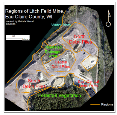
Figure 1: Study Area Map

The October and March datasets are not entirely the same. Between the two times, many of the piles have either been extracted from or added to, and some piles have been removed completely while some new piles have also been added.  That being said, there are still features between the datasets which allow for tie points to be established for the May data, as well as check-point features Which will be used to compute the root mean square error for each set of data.

Methods

Data sets involved in analysis

For this comparative survey, 3 flights were used for this survey which employed two separate platforms on three different days.  Here is a list of the flights ran

March: DJI Hexicoptor mounted with a Sony ILCE 6000 camera, set at 12 megapixel resolution. For processing one flight used TiePoints, and another project was created where only the GeoSnap was used for geolocation.

May and October: DJI Phantom with built in camera at 12 megapixels.  Both the data sets that used this platform set up had GCP's.  The October data made use of 8 GCPs while the May data made use of 15.

In an ideal situation, all of these data-sets would have GCP's attributed to them as a means for comparing the data to the same area that is not further georeferenced, but unfortunately on the day of the March 28th flight, the TopCon survey GPS was not working.  Because of this, tie points from the previous data set in October would have to be used to provide a more accurate georefference to the March flight.  As such, the first step to prepare the data for comparison is to process all of the data sets.  For the October flight,  the images were processed with GCPs which were allocated using GCP/tiepoint manager application in Pix4D.  After these GCPs were allocated, and all processing steps were complete, it was necessary to find features/objects present in both the March and October data to use as tie-points.  This is important because the March data does not have GCPs, and by using objects (tie-points) that are in the same location in as the October data will provide the improved geoaccuracy attributed to the October data to the March data. For comparative purposes, another dataset  was process with March data, but with no added tie points.  The fourth and final data set that will be apart of this dataset is the data collected by the phantom platform in March.  This data set has more GCPs than the phantom data from October, and the range of the GCPs is much broader.

Once the October data was georeferenced and the March data has completed initial processing, the tie points could be applied.  This process involves combing through both sets of imagery and identifying objects in the same location.  Once these object locations were found, a table of their locations was made based of of the UTM coordinates from the October data.  That table was than transferred into Pix4D and combined with each of the imagery from the flights in March.

Finding and Applying Check Points

In order to check the positional accuracy between each set of data, more features that are in the all the data sets must be identified and have their positions recorded from the October data. This process began by identifying 6 features with an adequate spread around AOI and recording their UTM location in the X,Y and Z directions.  These features were difficult to find, given that it was already a struggle to find matching features to use for tie points for the March data.  With that being said, the features were identified and applied.  The location of these points will be shown, relative to the GCPs used in the relevant data sets, in the results section (figure 2) 

Results and Discussion 

The results produced by this project yielded by this study were largely within the realm of what was expected in terms of the accuracy that was assigned to the various data sets based off of the processing method that was used for their geolocation. Below, in figure 2, is a visible representation of the offset between the check point feature and the processed location. below figure 2 are two tables that show the residual difference for each check point feature relative to the October data as well as the RMS error associated with each plane of direction (XY plane and Z plane)  

figure 2: Maps and visualizations of discrepancies between processed point and feature (bridge corner)

figure 3: figures associated with May GCP and October GCP accuracy

Figure 4: Figures associated with October GCP data and May tie point data accuracy

figure 5:  Figures associated with October GCP data and May 'no tie point or GCP' data accuracy

What was most shocking from this data is the fact that there was very little difference in overall accuracy between the data that used tie points to the one which only used the GeoSnap (Comparing figures 4 and 5). The only thing that made the GeoSnap data a little less accurate was slightly a higher discrepancy in Z values.  What perhaps this exemplifies to us is how using tie points to provide increased geolocation can cause issues.  The reasons this could be are as follows

1. Tie points allow for more room for human error during the alignment process during initial processing.

2. In many instances, like this one, its difficult to find features that can be identified in both datasets across the whole extent of the AOI.  Clusters of these tie points relative to areas where there are none will cause irregularities.

3. As a user becomes more desperate for features to use as tie points, they start to use features with less acute features, which causes the tieing-down-process to be less effective.

Their are ways to account for this accuracy drop off.  One way is to implore a camera or camera setting that uses a higher pixelation value, which would allow for features to be seen better and larger scales, allowing the user to allocate tie points better.  Overall though, this process is not nearly as trustworthy as using GCP markers, but often time requires the same resource expenditure associated with data processed with GCP's, because at some point, the data had to have been geolocated using GCPs.

The GCP method is much more reliable and increasing the accuracy of the data because the collectors have total control of the spread and the amount of points they chose to use.  This flexibility allows for ample spread to be applied, where as with tie points the users is highly limited to what features are distinguishable in both sets of data.

Conclusion 

Summary of average RMSE results:

8 GCPs to GeoSnap: .656 meters

8 GCPs to TiePoint : .653 meters

8 GCPs to 15 GCPs: . 260 meters 

Based off of these findings, if a company or organization is comfortable with having a potential discrepancy around .7 meters, using a UAS with a GeoSnap or a similar on bored GPS unit will suffice as means to cut labor and equipment cost.  However, if that accuracy does not provide adequate conditions to conduct volumetric analysis, the best scenario to use data that incorporates GCP's into the processing of the data.  One thing that is almost certain, is that these UAS based GPS devices will only get strong and more accurate, and will be able to provide ample accuracy without needing to apply ground control points/tie points.  This will prove to be huge because not all AOI's ace the same. The Litchfield Mine is overall, very flat, with little vegetation, and has a lot of free space to place GCPs.  Its unfair to assume that this will always be the case, and as such, its good to know that their is technology available that can provide sub-meter accuracy in a 3 dimensions  

Lab 8: Calculating and Comparing Volumetric Analysis Methods in Pix4D and ESRI Software.

Introduction 

Within the growing industry of geospatial technology, volumetric analyses is becoming a highly used application as companies start seeing the value such operations provide them in both accuracy and cost effectiveness.  Of the various industries that are beginning to employ its uses, the mining, construction, and materials industries are the the industries in Wisconsin which are using the most.  The technology allows for companies to know how much material is being extracted, transferred, and applied, with a higher degree of accuracy and efficiency than traditional methods.  The data that will be used in this lab was imagery collected from a UAS mounted with a high resolution camera.  Once the individual images have all been tied together into an geo-accurate orthomosaic, volumetric analyses can be conducted.  In previous labs, students conducted all volumetric analyses in PIX4D, and were essentially given the freedom to conduct volumetrics on anything in the AOI, which was a soccer field with a track around it.  In this lab, volumetrics will be conducted using both Pix4D and ESRI Software, and the volumetric results of three separate piles will ultimately be compared.  

Study Area

Figure 1: Litchfeild Mine and Piles for volumetrics

The area where this volumetric analyses will be conducted is the Litchfeild Mine, an active materials mine that is owned by the Kreamer Construction Company.  Relative to the city of Eau Claire, the site is located just south of town and is roughly a 10 minute drive from the campus.  Figure 1 to the right shows the totality of the sight as well as the three piles which will have the volumetrics calculated for.    The imagery for this map was captured using a hexicopter mounted with kinematic (RTK) GPS system and a Sony A6000 Camera.  The flight mission took pictures at 200 feet off of the ground at 24 megapixels.  The orthomosaic that was created as a result of this flight used 301 images, almost all were able to be calibrated to be apart of the orthomosaic.    

The Litchfeild mine has a number of piles apart from the ones selected for this  analyses.  between the piles, the land is uniformly level, allowing for the heavy machinery to pass through unopposed of difficult terrain or obstacles.  If students were at the sight when machines were operating on materials, they class would have to be equipped with MSHA certified clothing and hardhats, while also being guided by an employee of the Kreamer Company who was certified MSHA.  Safety is a very important aspect to consider when on a mining sight, as they can be very dangerous. 

When highly accurate data is desired, like in mining operations, the common practice is to use a dual frequency survey grade GPS unit to place ground control points to increase the accuracy of the orthomosaic during post processing.  However, on the day this data was collected, there TopCon GPS unit was not working.  However, there is a way to still provide further accuracy in this situation and this technique, known as using tie-points, will be discussed further in the methods.  

Methods

Before volumetrics can be conducted, the images must be processed and properly geolocated.  On the day that the data was collected, the TopCon Survey GPS failed and thus gcp points could not be obtained.  Luckily, there was dataset from October of 2015 that had been optimized with GCP points, and from that data set a table of tie point locations could be created.  Tie-points are land/structure attributes that are in the same location in both sets of imagery.  By importing the table of tie-points coordinates from the October dataset into Pix4d's GCP and Tie-Point Manager, the user can effectively use those objects which are in the same location in both sets of imagery as make shift GCP points. It should be noted, however, that in an ideal situation, the TopCon unit would have worked and we could have laid out the vast spread of GCP markers that the class showed up intending to do.  Had the class been able to do this, the output orthomosaic and point cloud would have been even more accurate. Figure 2 below shows the RMS error produced from this Pix4D projects from using these tie-points.

figure 2:  The RMS reports associated with the 24MP imagery at 200 ft using 4 tie points

figure 4: Volumetrics in Pix4D

Processing Volumetrics in Pix4D

Conducting volumetrics within Pix4D, the software that of course processed all of the imagery to this point, is a very user-friendly and straight forward task.  Like digitizing a polygon any other GIS software, creating a volume measurement in Pix4D requires one to click around the edges of a given pile.  Once the polygon is complete, the user can add, adjust, or omit vertices that have created the plane that surround the pile.  Once the volume plane has been created, the user can 'update measurements' with a simple click, and list of values are produced pertaining to the specific volume object selected.  A new feature of the updated Pix4D is a 'Base Surface Setting' menu, which enables the user to adjust certain aspects that ultimately affect the measuring parameters of  a pile.  Figure 3, to the right, shows the pix4D interface that is shown when a surface is created. At the top of the image are the measurement figures, which provide geometric properties of the pile created, as well as projected error and number of vertices used in the pile.  Below that, is the Base Surface Settings menu.  Here the user can change certain aspects that mainly pertain to the elevation and plane created from the surface polygon which encircles the pile.  A very hand tool that comes from this menu is the 'Align with  with lowest point' which levels the plane of the polygon created to of the surface to the lowest point, which could be helpful when calculating volumes that are placed on non flat plane.  The default parameter for this selection of settings is 'Triangulated' which connects all the vertices and triangulates the volume based on relative heights above/below the base surface. At the very bottom of the surface interface is the 'Images' pane.  Here, a user can scroll through and see all the images that have surface either completely or partially in that images field of view. Using the scroll bar on the right, one can scroll up and down and select a desired image, and from there zoom in and out / pan left and right within that specific image.  Not pictured in this figure, but no less useful, is the ray cloud viewer which allows the user to scroll through and pan around the 3D map created from the initial processing. Overall, this interface is very well organized and designed in such a way that it using the software requires little, if any, instruction at all.  It is very intuitive and sleek in its design, especially with the features that were introduced with the new update.

Calculating Volumes in ESRI Software - Raster Mask

The first of the two methods that were employed using ESRI software involved clipping a raster around the specific pile profile in the DSM produced in Pix4D.  Within ArcMap the specific extension that was used to conduct this analyses was 3D analyst.  Similar to the process of creating the volumes in Pix4D, the first step was to create polygon clippings around the piles.  Unlike in Pix4D however, the polygon created in ESRI need not be as tight to the edges of the pile.  Once the three polygons have been created around the pile, the Extract by Mask Tool is used to cut out the area of the DSM contained within the polygons created prior.  What is left from this operation are three chunks of the previous complete raster that contain only the piles that of interest.  Once the piles have been isolated, the user needs to use the identify tool to measure get the lands mean sea level height around the piles.  This value will be needed for the process of calculating the volumes of the piles, which is the next step.  Also, it is important to note that this is why the the polygon created around the pile should be loosely around the pile, not directly up to the edges, so that there is room to identify the height of the ground surrounding the pile.

Now that clippings of the DSM have been created, the volumes can be calculated using the Surface Volume Tool. Unlike with the last tool, which produced raster features of the isolated piles, this tool will produce a table with the volume and various 2D and 3D characteristics of each pile. Using the identify tool, input the flat height of the area around the pile and int the Plane Height input of the tool.  Figure 5 below shows what the inputs of this tool look like for the Surface Volume Tool.

Figure 5: Surface Volume Tool

Calculating Volumes in ESRI Software - TIN 

The final method for calculating the volumes of the three piles was by creating a Triangulated Irregular Network (TIN) out of the clipped raster piles. A tin takes the points produced in the digital surface model and coagulates them with an algorithm that turns the point cloud into a grouping of triangle planes.  Creating a TIN(s) is done using the tool Raster to TIN Tool, and calculated using the Add Surface Information Tool. These tools, in coordination with one another, ultimately create a field within the original shape file that surrounds each individual pile that contains that volume produced by the data contained within the TIN.  Below in figure 6, is an example of the attribute  table of one of the piles once both these tools were ran.  The attribute table for each pile looks the same, with different values, since the same process that were used to create the values viewed in the figure were conducted on each pile.

Figure 6: Geometric attributes added after data was processed through Raster to Tin and Add Surface Information, Tools.

Now that all three processes have been completed, the results will be discussed and concluded upon with speculative comments on what potentially could have caused the discrepancies between the pile volumes for each pile that was produced using the different software packages and methods.

Results and Discussion

Below, in figure 7, is a table that shows pile sizes of each pile that was created using each of the three methods. As one can see, there is a large difference between each method.  Based off of these results, the most accurate measurements are likely those that were produced by Pix4D.  In fairness, the software package apart of the Pix4D is more tailored for applications like measuring volumes of piles produced on mining sights.  Establishing the plane from which to conduct the volume measurements allows for allot more precise/customizable input, where as in ESRI, you have to more or less establish the entire plane based off of identifying the cell values around the base of the pile, which allows for inconsistent and very much random results, to be produced.  This is likely why the values for ESRI Raster Volume method are sometimes higher and at other times lower than the value produced in Pix4d. Similarly, the TIN values produced are all higher than the ESRI Raster Volume and ESRI TIN Volume for the same reason, the input parameters available are much less inclusive than that of Pix4d.  The options available for establishing the measuring plane are either the max z, min z, or mean z, which is not very realistic, because in the real word these piles could be laying on on slants, or be connected to another pile of different material that will throw off the mean z value.

figure 7: Comparative volumes of each pile using the ESRI and Pix4D.

For reference of what these piles actually look like, below in figure 8 is a map that displays what these piles look like relative to one another and the surrounding landscape. Within the map are images of the piles as they are presented in both Pix4D and ESRI packages.

Figure 8: ESRI and Pix4D views of piles and subsequent recorded volumes. 

Conclusion 

This lab focus's on the using three different methods sing both Pix4D and ESRI products to do volumetrics for comparative results has shown a contrast how these two software packages compare in this specific application of volumetrics. Pix4D, as their superior results indicate, is designed with this being a corner stone application within its software.  ArcMap, on the other hand, has a much broader spectrum of applications within GIS and remote sensing application, and so a drop off in accuracy is somewhat expected.  The same conclusion also applies for working with the data prior too producing any sort of volumetric results.  With Pix4D, working with the data is seamless and very self explanatory as you can process and conduct the volumetric analyses all in the same interface.  With ESRI methods, the process of creating the volumetrics takes several more steps and produce the values.  Thus, in the regards of ease and efficiency, using UAS remote sensing data analyses to produce volumetric measurements, for the very purpose of it being all inclusive and highly accurate.  ArcMap does have Drone2Map software that allows one to process UAS data, but that is another coast for an already expensive platform. 

Activity Day: Thermal Sensor on UAS for Detecting Humans and Various Thermal Signatures

Introduction

figure 1: Dr Hupy establishing connections while
Zac enjoys a cold one. 

On April 18, 2016, Dr. Hupy's UAS class went to the student Scott Nesbit's house in Fall Creek, WI, to conduct remote sensing analyses with an unmanned aerial device mounted with a thermal sensor. In total, 6 flights were conducted in the day, with the first flight being at 6AM and the last flight at 6PM. The purpose of these flights was to collect data for students Scott Nesbit and Zach Nemeth, whose research projects pertain to the uses and value of thermal sensor based data that can be obtained with a UAS.  Dr. Hupy, Scott, and the classes TA Mike Bommer needed to do multiple flights for Scott's project, and the rest of the class joined from 3PM to 6PM to help, observe, and gain more experience with setting up and running field collection operations with UAV's.

Zach's Project: Detecting Humans Using a UAS Mounted with Thermal Camera. 

Zach's interest is exploring the value of using a UAS platform mounted with a thermal sensor to detect human heat signatures.  The application of a project like this could elude to potential uses for UAS usage in cases of missing persons or criminal pursuits.  For his data, Zach had students and Dr. Hupy go throughout the area of the established flight which covered a portion of Scott's property.  Students placed themselves in a variety of land cover types: Tall grass, bare cornfield, under shade, and right next to a body of water ( small creek).  Diversifying the land cover is intended to get a better idea of the extent and capabilities of the thermal sensor.  When processed, Zach will classify the various temperatures that were collected in such a way that highlights the location of the persons scattered throughout the area.  

Scott's Project: Analyzing Changing Heat Signatures of Various Materials Overtime. 

Scott's goal was to use the thermal sensor to track the changing temperatures of various material and land covers throughout a 12 hour span.  For Scott's data, flights were conducted at 6AM, 9AM, Noon, 3PM, and 6PM.  Doing this, persumptively, was to create a contrast of heat signatures that various objects of interest would produce as time went on and as the temperature of that day fluctuated.  That day was rather warm, with a high amount of sun exposure.  For each flight that was conducted, Scott would use a thermal laser thermometer to get a temperature reading of the specific surfaces/materials that were apart of his study.  This was done so that the later on the appropriate sybologocial elements could be better tied to a precise temperature reading. The expectation is that these various materials will react to the different conditions throughout the day at various rates, some will cool and heat up faster/slower than other materials

Conclusion

This field activity was yet another opportunity for the class to gain experience with conducting UAS operations in the field. It was enjoyable to be out and about on the warmest day of this new spring, and it felt good to be made even more comfortable with conducting flight missions.  The biggest take away from this day in the field was a becoming more familiar with the pref light and post flight checklist.

Activity Day: Laying GCP's at Litchfield Mine

Laying New GCP's at Litchfield Mine 

On April 12th between the hours of 3 and 6 pm, Jo Hupy's spring UAS class, with the guidance of Kreamer Company Employee, Nicholas Kreamer, laid out 23 ground control points throughout the Litchfieled materials mine.  The mine is run and operated by the Kreamer Company, a native Wisconsin construction contractor that does construction throughout the country.  The weather was not cold for this activity, but the wind was rather intense, and was gusting hard enough to knock the hard hat right off your head, which happened to multiple occasions to multiple students.   

The intent of this activity was to lay sturdy ground control points there that could stand the tests of time, as well as highly intensive industrial activity.  The control points were constructed by the class the week before at the Hupy household, where students used spray paint on 2 ft x 2ft squares to make to create easily distinguishable colored patterns on top of the individual pieces.  The desgines made were two triangles that met in the middle of the plaque, each with a bright neon yellow color for a fill.  Each piece was also giving a letter identifier, which was also spray painted on, ranging from A to W.  

Lastly, each piece had four wholes drilled into it so that it could be nailed flat into the ground.  This assured the positions would remain consistent and not be moved by weather elements or the heavy machinery which would be operating in the surrounding area.  Just as well, because of all the heavy mobile machinery that operated at the mine, it was necessary to to have the control points of be made of a pliable material, so that they would not break if they were run over.  The material selected, as such, was a durable plastic, that if laid flat, would not break of become warped if ran over by the machinery on sight. 

below, in figure 1, is a map of the GCP locations relative to imagery that was captured in October 2015.

figure 1: GCP marker locations

This activity will allows for missions to me conducted repetidly at this location without having to continually relay GCP makers, making it much more less logisticaly difficult going forward for UAS classes of the future. Just as well, A fast and easy way to create home made GCPs was created in the process, which could be prove to be useful when out of school in a professional setting. 

Lab 7: Project Proposal - Volumetric Calculations Using Imagery Gathered with an Unmanned Aerial System Equipped with High Precision GPS vs Imagery that Uses GCPs derived from Survery Grade GPS Units

Introduction  

The project that will be briefly outlined in this post will discuss the research of to how to use tie points in conjunction with GCPs to create a geo-accurate imagery, from flights done at separate times over the same area.  Subsequently, with that geoaccurate product produced in the computer software, Pix4D, volumetric analyses will be conducted on multiple debris piles. These measurements will be conducted on imagery produced by 3 separate flights flown on the same day at varying heights and varying resolutions.   Once these geoaccurate products are produced, and volumetric of the various piles are made, maps will be made to show the variation between the flights that were conducted on that day, with a map being made for each unique height/resolution combination. There will be three in total. 

Study Area

The maps that will be created will display the results of research that involves unmanned aerial systems that are equipped with commercial grade, highly accurate real time kinematic (RTK) global positioning satellite (GPS) system, as well as a digital Sony A6000 camera.  When highly accuracy data is desired in most UAS operations, the common practice is to use Dual Frequency survey grade GPS units are used to place ground markers which are than used to create Ground Control Points (GCPs), which are than incorporated into the image processing in the Pix4D software to provide maximum accuracy. However, This method adds considerable cost and time to collecting data with a UAS.  For the sake of this research,  This UAS  imagery will be post-processed using Pix4D software to generate digital terrain models, which will then brought into ESRI software for further analysis.   The ultimate result will be a series of volumetric analyses, where results will be compared between imagery using the UAS High Precision GPS and imagery corrected with GCPs produced by Dual Frequency GPS units. 


The area where this study will be conducted at the Litchfield Mine, a sight that is operated by the Kreamer Brothers construction company.  This sight has a number of piles of varying material types.  The area which these piles are held is enclosed by forest, a retention pond, and a bike trail.  Figure 1 below provides a map of what this area looked like on October 15th of 2015.  The data that will be used to create the volumetrics for this research, however, was collected on March 13, 2016 between 11:00AM and 2:00PM.  The day was overcast with little wind,  which provided great flying and photographic conditions since there was little shadow as a result of low sun exposure.

figure 1: Litchfield Mine Study Area

Methods

The methods that will be used in this lab will be, in part, similar to that of previous labs.   This is because this research will incorporate multiple projects that will ultimately be cross analyzed to compare results, some in methodologies which we have used prior, and some that are brand new.  In essence, three approaches will be taken to provide the results which will ultimately be used to create volumetric comparisons.  Here are the approaches that will be taken:


1. Straight forward processing, relying only on the geolocation provided by the high quality GPS that is on bored of the platform.

2. Processing with Tie points/GCPS.  This approach will incorporate GCP's locations that were recorded at a previous time, while combining those points with tie points that were collected by matching up the locations of visible features that are present in both sets of data - objects that are visible in the data from march and also the data from October.

3. Process the imagery with only GCPs but no tie points to derived from objects that are consistent in both sets of imagery.


Ultimately, regardless of the set of methods used, the final product will be exported into ESRI software for volumetric analyses to be conducted.  Important things to compare as a result of this operation will not only be the sizes of the piles derived from each set of data, but also the amount of root mean squared error that is attributed to the calculations of each pile, relative to that of the same pile produced using another method.

Discussion

Will need to know more about the results to fully discuss the varying datasets and methods used in this research. 

Conclusion

This section will discuss the findings of the research and identify weather or not using high grade GPS and camera equipment on bored the UAS platform provides enough accuracy to eliminate the need to collect GCP points while collecting imagery.  The upfront coast of this technology would be more, but overtime would save money by reducing the labor cost of placing the GCP points and the material cost of cr

Lab 6: Class Flight with Matrix UAS Platform - Thermal Sensor

Introduction.  

There are those days where as a Wisconsinite you wake up and just feel amazing.  The first thing you hear, birds.  The first thing you feel, warm sun coming through a window.  An emidiate energy that you feel only a few times during a Midwestern window.  This was the first day it really felt nice again.  As such, our professor did not hesitate to take the opportunity to take advantage of the conditions to get our class some time observing and partially participating in a flight mission while also getting the chance to test out a new sensor that is still being configured by the department, a new thermal sensor.  

In fact, I was lucky enough on this day to experience 2 trips to the field. Both times involving unmanned aerial systems.  In all, I learned a lot about how to establish a safe environment for flying a drone.  The aspects that you must continually monitor when flying a drone is the drone itself, the people around, and the environment of the flight mission. To ensure that all these conditions are ideal, there is an extensive checklist that the pilot and the co-pilot must conduct before each and every flight. 

In the sections that follow, I will discuss the operations conducted and things I learned during this field experience in terms of lab procedures and field methods.  All in all, the focal point of this activity was to gain field experience with the Matrix Platform, and all the other electronic components that relate information to and from the device before and during the mission.  

Methods

Before any flight operation, even the mission comes only minutes after flying a previous mission, its imperative that the UAV be given a thorough check down.  This list can very from only few basic checking points, to a long list of safe guards (recommended).  In the case of these flights, the pilot was the classes teaching assistant Mike Bomber  and his co-pilot was our Prof. Jo Hupy. Over time and through many flights, these two have developed a checklist that accounts for checking the drone of any hardware issues, making sure all the systems are connected, while also providing a cleared areas for both take off and landing. 

Multi-Copter Check List 

The Matrix platform that we are used in the field for this this session was the Matrix Platform equipped with a Geo-snap and a Grayscale thermal sensor.  The Matrix a quad-copter with its propellers mounted in rectangle relative to one another.  As such, the centrifuge mount of the device is long, almost looking like the chasi of a car. To conduct the checklist of this specific platform, a hard cased field laptop was to open up an excel document, which contained the check listed information.  The co-pilot went down through the components of the checklist, reading them out loud to the pilot, whom is will eventually be holding the TX controls, but is right now responding to the calls from the copilot and doing the necessary checks. 

When flying a UAV, your checklists will differentiate depending on what type of platform you are flying (fixed wing or copter) and also between platform types within their own respective groups (Matrix vs. Phantom).  The checklist for multi rotors was broken down as follows: 

1. Mission conditions and flight prep 

2. power up 

3. take off sequencing 

4. post landing

Each component its own way is important when trying to conduct both a safe and successful mission, that provides meaningful results while also lowering risk of damages. Lets look at these individual portions of the checklist more closely.  

Mission Conditions and flight prep 

figure 1: environment conditions and flight prep

The first component of the checklist, the conditions and flight prep is done so that any conditions that could be detrimental to a flight mission can hopefully be identified.   The focal point of these checks are to find any sore of hardware issues that if left undetected, could cause a huge problem during flight time.  As the co-pilot reads down the list, the pilot is checking the part being called to them for any cracks, looseness, or other issues they notice.  Another thing that is noted of during this check are the weather and environmental conditions of that area of interest during that time.  This is important to note for when you are processing your data and notice any particular issues with data or image quality, for the issues could be related to conditions. 

Power up

figure 2: power up checks

The power up check occurs after the platform has been checked for damages and the environment scanned and cleared.  This check assures that all the devices are in connection with one other while also checking to see that each component is connected on the platform, and that the battery is providing enough voltage to supply the components of the platform with enough power.  Another notable thing that is noted here is the GPS signal strength. This row can bee seen highlighted by the green and yellow in blocks in the row titled UAS # of Satellites. Having more satellites tied to your location is best, because it provides more vantage points to your position and increases your positional accuracy.

The penultimate part of the list accounts for sending all the appropriate information to the platform, so that the device has the necessary flight path and altitude for its mission.  This process can be skipped, however, if the flight is being conducted manually, and thus you would not need to send any mission to the mission control aboard the platform

Take off Sequencing 

figure 3: Final checks before take off

Before taking off, the final portion of the checklist, the final components are armed and the controls are engaged.  after all necessary connections are made, and the controls are in the hand of the pilot and the right commands are being produced, the fight is almost ready to begin.  The last step is once again making sure all spectators are clear to launch.  Once the pilot takes the device off the ground by pushing the left stick up, the pilot than turns the device onto loiter mode, where it will hold its position and not move horizontally or laterally. Once here, the pilot than gives the control with another switch to engage mission, and just like that the device takes off and goes to assigned start point and begins its mission. 

Post Landing 

figure 4: Post Landing checklist

Shortly after landing, when the power has been turned down the motors are stalled, the pilot and co-pilot can begin their final check.  This must be done even if more flights are still to be conducted later on.  This short list covers disconnecting all the components to isolate the device from any remote connections or power sources.  Once complete, the pilot checks the sensor to make sure it is still fixed in the position that was desired.  

Once disconnected, the rest is up to you.  If there are more flights planned, its likely that you have spare batteries ready to replace the ones just used during the flight.  If not, your day of collecting UAS data is likely finished.  At this point, you should go have nice lunch or drink to conclude a trip to the field where you didn't destroy any of your precious devices, all because your were thurogh in your pre and post flight check, Cheers!!!!

Results

Below is a map showing the subsequent tiffs created from the two areas we flew over during our time in the field on May 7th. The whole collection process took about 2 hours, and both of our flight mission ran smoothly.  within this map, you will notice that i focused in on certain areas of both the flight over the garden, and over the pond, to highlight certain aspects of the AOI and how it relates to the data quality provided by the sensor

figure 5: Maps of AOI and specific issues associated with thermal sensor

Discussion

Provided that the main purpose of the thermal sensor was to capture the relative heat differences across an AOI, the data didn't prove to be as useful for indexing features as I thought it wold.  For example, if you refer to the scaled image at the top right of the document, you will notice that there a car, but that is really it.  It is very hard to distinguish that the red objects, directly north of the car, are in fact warm bodied people.  I found this concerning, since throughout the pond image we had people scattered about, and they were very much unidentifiable.

I was wondering if this is because of inadequacies within the sensor, or is it because it was one of the first warm days of the year, and the ground had been exposed to the sun all day.  Just as well, the AOI was covered in newly developed snow-melt puddles, which added alot of contrast to the surrounding ground.  As such, the AOI had a lot of varying elements with a wide ranged of temperatures attributed to the certain portions.

For the sensor, I believe that using it only nadir angles was very limiting in terms of detecting humans bodies.  This is because from up above, humans would only occupy a seemingly very small amount of space.  Perhaps, if taken at oblique angles, their would be more of a subject for the sensor to pick up, because there is more available human body to take heat readings from.  If the purpose is detect heat sources, and not produce an accurate orthomosaic, this might be the best approach going forward in terms of increasing the ability to detect humans as the subject of thermal imagery.

The last concern I had was in the DSM of the pond area, and if you refer to the image in the bottom right of figure 5, you can see what i am talking about.  The area being focused on is the actual water body of the pond.  This could be patches of remaining ice floating above the water which is why the image appears to be oddly ridged at the center of the image.  However, this could also be as a result of the sensor being not very good at getting a good reading of water bodies.

Conclusion

The value of this lab was rooted in the experience of being able to observe a full flight mission on beautiful spring day.  I learned the amount of caution one must approach all UAV flights with.  If always cautious and diligent with your premade checklist, you will hopefully be able to detect any malfunctions before they become mid-flight catastrophes.  Not only that, it was also help full to see the order of operations in terms of creating a mission plan, exporting the mission to the Matrix platform, and executing the mission.

In terms of the data, I am not sold on the data quality of the imagery obtained from the thermal sensor.  It was to difficult to see any true heat coming from the human locations on the map.  That was a concern.  Again, I am not sure if this can be improved upon by better mission planning, where if we know the subjects that we are looking for, we adjust the mission accordingly.  For example, I believe these results could have been made better had the mission been conducted obliques. 

 

Lab 5: Using Oblique and Nadir Data to Create 3D Models.

Introduction 

Imagery collected from UAVs can be either oblique or nadir, and both have varying applications and uses with the remote sensing industry.  Nadir, implies that the imagery was taken at or very near a perpendicular angle to the surface below.  Oblique imagery is when the focus of the image is both below and to the side of the sensor, creating a more profiled view of the area/structure being observed.  So far for the labs in this course, students have worked almost exclusively with nadir imagery.  In this lab, however, both types of imagery will be utilized and merged into one in order to create accurate 3D models.  

There are two types of oblique imagery, high oblique and low oblique.  Low oblique implies that the horizon is in the view of the image.  When creating low oblique data-sets, its imperative that the images are captured with the horizon at 180 degree angle relative to the edges of the frame, simply because that is how we has humans expect to view the horizon.  High obliques, on the other hand, are taken at larger angles relative to the ground and do not show the horizon.  Because the horizon is not in view, there is not as much importance of capturing images parallel to the horizon.

In terms of industry uses, Nadir imagery is what is primarily relied upon for creating geoaccurate products like orthomosaics and DSMs.  Oblique imagery is more or less used to for photographic aesthetics because it can provide unique angles that show angles that are pleasing to the eye. For example, in class we saw how oblique imagery was used to help create a 3D model of a construction site.  This technology, when compared across a temporal scale, can really show with great detail the progress of an changing area or structure because it allows the viewer to move across space and view the whole area at varying heights as well as angles. When used in conjunction, the geoacurate data from nadir vantage points combined with oblique imagery can add detail to areas desired, providing higher accuracy and detail at the same time. 

The focus of this lab is how a user can use both nadir and oblique imagery to create 3D models in Pix4D.  In doing this, a report will be produced that comments on the product created through the merger of these contrasting angles.  In conjunction with imagery itself, it will also be important to factor in how the conditions of that particular flight mission effect the output, as well as AOI being captured in the imagery. 

Area of Interest

The area of interest for the focal activity of this project, merging nadir and oblique imagery project to create a 3d model, is a farm.  The area has a number of structures, both small and large, the largest being barn.  The UAV missions that were conducted to collect both the nadir and oblique imagery sets took place in the winter, and much of the surfaces in the AOI are covered in snow.  When creating 3D model, its very important to understand how the landscape itself will effect the quality of a project, and adjust accordingly.  Now, given that this is sample data that was given to us, we as students did not have the ability to take this into consideration and create a plan of action.  Had we the opportunity, it would be important to confider the following. 

• Because the landscape is snowy, a higher degree of overlap will be necessary 
• recommended overlap - Frontal: 85%  Side; 75%
• set sensor settings accordingly to maximize contrast in the AOI imagery.

Now that we covered the specifics of the overall Area, the focal point of the 3D model is the next important thing to discuss - The Barn.  The barn is the object or structure in the AOI, and even though the nadir imagery captured images away from the barn, the oblique images (roughly 30) focused directly at the barn.  In this situation, as with any other oblique imagery taken for the purpose of creating, to create the best result possible you should try to use very diverse data.  Diverse, in this instance refers to imagery sets taken various angles and viewpoints.  The more vantage points available, the more accurate the resulting model can be.  Ideally, when working exclusively with UAV data, the nadir imagery involved should aim to provide vantage points at or near how it appears below in figure 1.

figure 1: Ideal oblique imagery vantage points.

In some cases, you can even add images taken at the ground level to add another layer of detail that isn't as available fro.m a UAV. This video shows just how in-depth the data collection process can be

Examples like this are highly data intensive, and as you can see, highly resource intensive. Let us consider this video when analyzing the project designed to capture and model our 3D barn.  Below, in figure 2 we can see the DSM and Orthomosaic produced by the final merged products with tie points included.

figure 2: Map overview of farm.

In reference to these maps, one can see how the land itself is predominately flat, with a slight slope approaching the south east.  On the land, their are a number of objects both natural and man made which obstruct from the relatively flat surface.  These items include buildings, trees, machines, and other structures.  From this overhead nadir position, we can also see that the farm is cornered in by a road that is to both its east and south.  The road runs north south and turns via an elbow to a east/west orientation.  Within the area contained by the road we see a number of structures, including a barn, a triple set of silos, a house, and several garages.  The tallest portion of the area are the three silos, visible as the cluster of three white circles in the DSM map.  The other tall objects that seem oddly shaped along the outskirts of the farm area, by the road, are trees.  As mentioned before, because the season is winter, snow could potentially be on top f any of these structures, as well as the land, which it clearly is.  As such, height values could either be the actual height or the height of the snow which is on top of the normal surface. 

Methods

To create a 3D model project out of two previously made projects, there are a few extra steps involved as one would expect.  To get these projects ready to merge, initial processing needs to be completed on both an oblique set of images and a nadir set of images.  In the case of the Barn Project, we had about 150 nadir images and roughly 30 oblique images. Once initial processing for those two separate projects has been completed, they can be merged together to create a 3D model project.  Since both sets of images were created using the same sensor, the sensor specifications match up easily. The important thing to remember is to use 'distance above WGS ellipsoid' for the input ordinate system z values and the output z coordinates to be mean sea level.

3D model of Park Pavilion - Soccer Park

Creating the 3D model of the park was simple, but the product was not very sharp.  This mission when ran was only done using almost exclusively oblique imagery, and very little from over head nadir positions. As such, you have varying levels of distortion around the area of intrest, both on the pavilion itself or in the area surrounding it.  The distortion of area around the pavillion makes sense, mainly because it was for the most part captures as foreground to the pavilion.  Whats most concerning is the distortion of the subject of our AOI, the pavilion.  Figure 2 exemplifies this distortion, and can be seen below. 

figure 2: Park Pavilion - notice distortion from prodomenetly oblique mission. 

Creating in 3D model in pix4D does not create an orthomosiac or DSM, like what you can create when building a 3D map.  As such, there is no format in which it could be brought into ArcMap. Without these two things, geolocation is not reliable in any means, and cannot be worked outside Pix4D in mapping programs, like ArcMap. 

Nadir and Oblique Merge Project - Winter Farm Land 

The merged project of nadir and oblique imagery of the winter farm land produced better results, but still left more to be desired int terms of quality.  What popped out that was initially a concern, was that the merged project layers didn't overlap and stack perfectly, there seemed to be two floating just atop one anther.  Figure 4 below exemplifies what I'm talking about in this instance. 

Figure 4: Side profile of unoptimized data produced from merged oblique and nadir image sets. 

To create a better representation of the AOI, manual tie points were added too areas where the two projects overlapped the most, around the barn.  Three tie points were added to visible corner features that were apart of the barn.  Each tie point created used roughly 20 images to calibrate a location for the tie point.  The key with this process, is to make sure that the tie point is adjusted in both imagery taken from the nadir and oblique imagery set. Doing this will correct the unwanted layering that was present after this project was completed without GCPs. figure 5 below shows the location and orientation of these tie points in relation to the barn structure.

figure 5: Tie points used on barn.

Once the tie points are established, re-optimization can be conducted.  In this instance, I re-optimized by initially only rerunning the initial processing.  Once that was complete, and I could see the results produced, I was confident that i could  ran the point cloud and mesh, as well as the DSM/Orthomosaic re-optimization and produce a better product than what was created initially. When the orthomosaic was complete, what i thought would be a properly aligned merge turned out to still not be 100% correct.  Figure 6 below shows the adjustment that took place after the tie points were applied in the optimization process (compare with figure 4).

figure 6. Barn distortion post tie point application and re-optimization. 

What i believe occurred here, and i must admit that this was an oversight on my part, but I should have used a broader range of Tie points.  What i mean by this, I should have used more than 3 and I should not have had them so clustered.  My thinking was that i only needed to put tie points on the barn because that was the area that intended to be the focal point of both projects that were merged.  What i should have done is added more tie points to things on the ground, which would allow the orthomosaic to calibrate and better synchronize the merging projects' z values.  With a larger spread of tie points, this data could be even further optimized.  

Discussion

Nadir and oblique merge project

To create a meaningful 3D project, the data acquisition process must be concise, thorough and optimized.  In this instance, merging two data sets into one showed how issues can arise and alter your data in ways not expected.  In the last lab we as students conducted for this lab, we learned the power of using GCP points to re-orientate data to provide maximum accuracy over an area.  This, as we found out, is even more so important when creating a project from two separate flight missions. Just as in the last lab, laying down manual tie points and optimizing the project was the key to creating a meaningful product. 

One issue that could also have produced better results is by adding a more diverse range of data to cover the pavilion that is being modeled.  As we learned from the pix4D sponsored video shown above, the more data and vantage points the better.  In comparing the two projects, redoing this project with both GCPs and more imagery (at both nadir, high oblique and low oblique) would likely produce a better result then what observed.

Pavilion 3D model project

In terms of the distortion involved with the modeled pavilion, several things could account for to the predominantly distorted project that was created previously.  In either case, there is likely more than source of distortion at play , and I would ascertain that the distortion was a result of a a combination of these possible errors: 

1. Sun distortion 
2. inadequate coverage by sensor 
3. Varying landscape in foreground 
4. Sensor malfunction
5. GPS malfunction.  
6. Lack of GCPs could have resulted in insufficient calibration of images

Of these potential causes, I believe 1, 3, and 5 to be the most likely contributes to the distortion we see in the the pavilion. Sun distortion likely played a factor because the pavilion has a relatively dark and metallic roof, with various angles.  This could cause sun light and heat to interfere with the data collection process.  The evidence for this can be seen in the portions of pavilion that seem to melt, a typical sign sun distortion. Also, when the foreground of an oblique image is constantly changing, the software has less common ground between images to match during the overlap process when creating the 3D mesh.  As a result we get the level of pixilation at various part of the modeled pavilion that can seen in figure 2 back up in the methods section.

 Referring to the quality report, one major concern I saw in the quality check was that only 48% of the 188 images were able to be calibrated by the software. That means that over half of the images were thrown out because they could not be appropriately geolocated. What could have helped calibrate these images would have been by using GCPs.  Had they been used, there would have been more overlapping data that could have been used to create a more complete and good looking model. figure 3 below shows the quality report created during the initial processing of this project.

Figure 7: Quality report for 3D model creation of pavilion

Conclusion 

Working with oblique imagery can be a tedious process in terms of both collecting and processing.  What has become apparent is that thoroughness is of a very high importance when trying to create a good 3D product.  To be able to use a 3D product, and benefit from it, one must be thorough in creating adequate overlap and geoaccuracy.  Doing so will help Pix4D be better able to accurately calibrate  the imagery, maximizing the efficiency of your flight missions.  It is simply a waste of time and resources if only half the data can be calibrated from a UAV mission because of inadequet georefernce or overlap.  Preventing this can only be accomplished if mission planning is prioritized to a high degree.  If rushed or not fully thought out, the product will provide nothing that is worth sharing or using.   As such, creating a good 3D map/model product is dependent on the mission planner providing a diverse array of vantage points as well as GCPs/tie points which allows the data to be better callobrated.

In relation to lab 4 (seen just below this lab), I should have done more of what i did in that lab in this one.  I should have spread out my tie points more and not have put them on one structure that occupied a very small amount of the total subject area.  Going forward, I will often refer to the lessons learned here so that I do not repeat being thorough with the necessary user input when processing imagery to create respectable 3D products.