Lab 4: Using GCPs in Pix4D

GCPs in Remote Sensing

The use of GCPs involve using raw data collected from on ground GPS system in coordinate with images that have assigned spatial attributes.  GCPs are intedned to provide extra spatial context to the data, allowing the final products to be more geometrically accurate than the the raw data collected with the sensor-gps systems. GCPs are used most in applications where high, often sub-meter accuracy,is needed. In order to incorporate GCPs into remotely sensed data, the GCPs and geo-accurate images me combined during initial processing, and are fine tuned by the user after the product has been produced.

Going forward, this blog post will pertain to the acute methods of how to appropriately use GCP points in the Pix4D software. Ultimatly, the discussion and conclusive data will be primarily focused on comparing an image product that uses GCP points, and the same data without any GCP points. The final result will be a set of maps, which will be the bases of comparison.

Along with describing the process of incorporating GCPs into imagery obtained using GeoSnap will be an overview of the common methods there are associated with using GCP points in Pix4D. In total, their are three and each have an their own advantages and disadvantages.  Often times, depending on the method, you are subtracting accuracy for time, or vise versa.

Methods

How to Integrare GCPs into a Project

Source of geographic accuracy can be called upon by utilizing a multitude of geo-accurate data sources. There is the topographic method, which is the survey method, where points are taken in the field with hardware and and imported into pix4D and combined with the imagery. Then, there is the method that utilizes data that is already considered to have a geographic level of accuracy.  Sources for this can be topographical - navigation maps. The final method, utilizes the accuracy from a Web Map Service.

Regardless of how these points are acquired, there are 3 distinguishable methods of how to use GCPs in pix4D.  The factors to concicer when using GCPs, are as such:

• If the initial images are geolocated or not
• The coordinate system of the original images 
• The coordinate systems of the GCPs

Depending on what combination of these factors you are dealing with in, in terms of your data, a user must choose which direction to go as for  how to integrate GCPs into their imagery.

Method A: images and GCPs have known coordinate systems 

This method is the most common.  It allows one to mark the GCPs on the images with little manual input. As such. this method is not suited for "over night" processing where all processing steps are initiated at once and can be ran all at once.

1. obtain GCP measurments from a device in the field
2. Import GCPs using 'GCP / Manual Tie Point Manager'.  Often times, the GCP attribute data requires that the data be massaged to the right format in order for it to be available for use 
3. On the menu bar, click Process > Local Processing. 
4. Activate Initial processing
5. Deactiveate the Point Cloud Mesh and DSM, Orthomosaic and Index options  
6. Click Start 
7. Mark GCPs with Ray Cloud
8. Analyze quality report

Method B: Initial image has no geolocation, initial images are geolacted in arbitrary coordinate system, or the GCPs are in an arbitrary coordinate system.

Method B allows users to mark the GCPs on the images with little user input, like in Method A.  However in this case the the images are not geolocated  and the the GCPs are geolocated useing an arbitrary coordinate system. Also, this method is not suited for "over night" processing where all processing steps are initiated at once and can be ran all at once.

1. Obtain your GCP measurements and have the in a proper location
2. allocate them to the proper coordinate system that best fits project
3. On the main menu bar, click process > local processing and only select: 1. Initial Processing. Do not select Point Mesh Cloud or Orthomosaic and Index.
4. Click start 
5. Add/import 3 GCPs with the Ray Cloud tool.
6. add extra GCPs obtained from field or tabular data into the software with ray cloud or GCP/Manual Tie Point. 
7. Remark All the GCPs with Ray Cloud.
8. Complete the final processing steps needed to complete the project (Point Mesh Cloud or Orthomosaic and Index).

Method C: Applies to any case 

Method C works for all cases and it does not matter what the coordinate sytem of the images or the GCPs are but it requires more user input to work the GCPs in the Images. The advantage of this method is that after importing the images and the GCPs, the processing can be done without any user input or attention and be left to conduct its long processing operations .

1. Obtain your GCP measurements and have the in a proper location
2. allocate them to the propper coordinate system that best fits project
3. Add/Import all of the GCPs with GCP/Maual Tie Point Manger 
4. Mark the the GCPs on the image with the BASIC GCP/Manual Tie Point Editor.
5. Click ok to close the GCP Editor.
6. Begin the "over night processing" of creating by running all three processing steps at once. 

The method the user selects is contingent upon what resources he/she has available and also the nature of the data they are working with. If the image has an assigned coordinate system, than the GCPs georefrence must match that of the imagery.  However, if the image has no georeference than the user can choose a use an arbitrary coordinate system for the GCPs.

Steps of Creating a Pix4D Prooject using GCPs with GeoSnap Imagery - An Overview

To create two comparable projects, one with GCPs and one without, for the project with GCPs, Method A was the method that was used.  However, before getting involved with the GCPs, there are several steps the user must preform in conjunction with GeoSnap data so that its images can be used by Pix4D.

Normalizing the picture in the georefrencrence file is the first step in this process.  Unlike when using the Cannon SX290 images in previously labs, the GeoSnap imagery  does not get uploaded into Pix4D with attributed spatial information assigned to it automatically.  Like with the GEMs, you must join the imagery with the Export file that is created when exported into Pix4D.  This file contains the rows and columns of spatial information that is needed to create a Pix4D project.  However, before these files can be used to accurately provide geolocation, the data must be massaged.  This is process is similar to normalization, but instead of having the correct name, all that matters is that you have the correct order of your columns. Figure 1 below shows what the massaged data looked like.

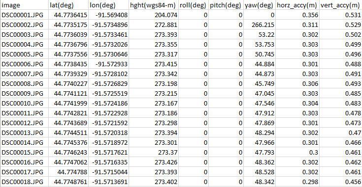
figure 1: Table in the appropriate format that can be read by Pix4D software.

To create this new formated table, the file was exported to Excel, where the columns were massaged in the right, proper order, and than reconverted back to text for use in Pix4D . Once this process is complete, the images can now be assigned accurately using the massaged table.

Next, the user must adjust a few parameters within the coordinate system advanced options.  The user must select Geod Height Above WGS 84 Ellipsoid  ( 0.00) for the vertical coordinate system.  The default coordinate system for the images is WGS.  However, a few steps later, the user is advised to select MSL (mean sea level) for the output coordinate system because that way it can be compared to USGS Data which typically uses MSL for there data format.

Now, the user can import their GCPs.  First, its impartive that the Geographic Coordinate System of the imagery and the GCPs are the same.  In this case, although the GCPs being imported into the software are in UTM Zone 15N, they still are still attributed the GCS geoid.  Once all requisit coordinate information is input into the system, the GCPs will display in the the GCP/Manual Tie Point Manger with all fields populated. By clicking Next, THE GCPs will than appear on the viewing interface, above the imagery, displayed as X's.  Once GCPs are in the system, initial processing can be ran.  This processing took roughly 2 hours to complete.

Once complete. Ray Cloud editor opens up allows users the ability to further increase the accuracy of their imagery.  When editing with the Ray Cloud Tool, the user can see a legend of all the GCPs and images that are associated with those GCPs on the left, and a smaller image pan on the right opens if one of the GCPs in the legend is selected.  When this imagery was taken, the data collectors place orange and white icons at the precise locations of the GCP points.  Using that in the right doc imagery pane, the user can adjust the GCP point location so that is more directly Centered at the center of the geoaccurate spot.  Figure 2 below shows what this pane looked like during the process of adjusting the GCP points. Each GCP had anyware between 17-25 images that captured it in part of the flight mission.  The user has to go through and adjust the GCP location for every image that is is found in, to create the most accurate product.

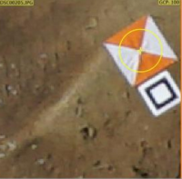
Figure 2:  The yellow cross hairs represents the GCP location and the orance and white structure represeant the a Geo-Accurate point.  The GCP will oftentimes not be centered at this point, and will be off of the point by several meters.  The user, like displayed in this picture, clicks and centers GCP point so that it is as close to the center of the geo-accurate marker as possible. 

This process is very simple though, and by zooming closer in on the image pane, the user can pinpoint the points with a higher degree accuracy.Once all of the images associated with each GCP is is adjusted using Ray Cloud Editor, the final steps of Point Cloud Mesh and DSM/Orthomosaic Index can be ran to complete the Pix4D project.

To create the same project without GCPs, the data was still massaged so that it would fit into Pix4D software, where all adjustments to the reference coordinate systems are done as specified earlier. This time round, however, all processing can be ran at once because no GCPs are being used.

Results

The maps and images shown in figure 3 indicate the different levels of accuracy between the orthomosaic that was created with and without GCPs.  The image to the right of the maps shows a geo-accurate ground point that was taken with a survey grade GPS device, the X represents how that GCP was shifted during the projection process. The bottom map/image display what each of the GCP points look like relative to the point on the actual ground.  This accuracy is established after initial processing when the Tie Point/ GCP manger was used to adjust the GCP point so that it was as close to center on the ground point. 

Figure 3: Orthomosaics with and without GCP points

Visibly, just looking at the maps doesn't really give any indication that there is a difference between the two maps, but when looking closer at the geo-accurate point in relation to the digital GCP, you can see that a shift does take place.  The mean shifting of each GCP point was roughly .96 meters in any direction.  This statistic is made available in the Absolute Geolaction Variance reports which can be refereed to in the next section, within figure 4.

Discussion 

Using the quality reports produced by both of these projects, one can observe if there is a difference between Geo-snap data with and without GCPs. As you can see the project with the GCPs produced a higher RMS error for the X, Y, and Z value, in comparison to the project with just raw Geo Snap data. The values being refereed too here, are the values represented in the bottom row of each figure.  This is interesting, because the maps created in ArcMap show how the orthomosaic that was realigned with GCPs was spatially more accurate.   

Figure 4: Absolute Geolocation Variance chart from Pix4D quality report - GCP Points

Figure 5: Absolute Geo-location Variance chart from Pix4D quality report - Raw Geo Snap data, No GCPs

This seemed counter intuitive, it seems that the in Pix4D the imagery things that report thinks that the images are accurate because the software thinks that the imagery is accurate, when in actuality the survey point in the image is the most accurate attribute, hence why we as users used them to adjust the GCP locations in tie point manger.

Because it is intuitively backwards,  The figure that should be payed attention to most is  mean (M) shift in geolcation ( figure 4 and 5).  Because Pix4D thinks its imagery is the most accurate source, it shows very large mean distance from actual location, for the x,y, and z components of each GCP.  Referring to the same statistic in figure 4, that same value represents the mean distance each GCP was shifted to make it so it lined up with the geo-accurate survey point. Each point had to be roughly moved 1 meter to be fit right above the center of the survey point.

Conclusion 

Using GCP points shifted the imagery to more accurate ground locations by roughly a meter overall. This shift is not noticeable at small scale comparison, but can be observed when taking a view at much larger scale factor. GCPs are very important tools that provide the means to create accurate imagery data that is in high demand for a number of growing industries.  Within industries, like construction and urban planning, being accurate to the meter is not enough.  In this world, centimeters measure the difference between a successful day of building and an  expensive redo. 

Lab 3: Processing Pix4D Imagery

Introduction - Part 1: Get familiar with the Product

What is the overlap needed for Pix4D to process imagery?

The recommended overlap used in Pix4D is 75%

What if the user is flying over sand/snow, or uniform fields?

When working with ununiform surfaces, it is recommended the overall overlap of images should be increased: minimal 85% frontal and 70% lateral.

What is Rapid Check?

Rapid Check reduces the resolution of the images used in a project from their original pixelation to 1MP.  As a result, operations can be run faster but as a result produces lower global accuracy because there are less overlapping pixels which can be match to one another because there are now less pixels per image.  This often done to check the overall quality of the data consumed by the device.

Can Pix4D process multiple flights? What does the pilot need to maintain if so?

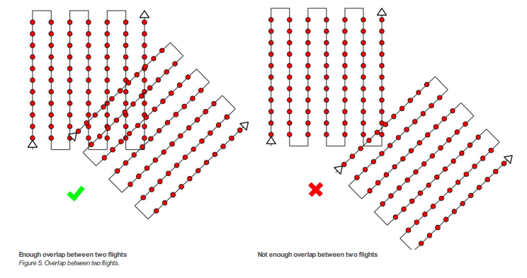
Pix4D can processed datasets composed of multiple flights provided that the total number of images is less then 2,000. Just as will the images from one dataset, when combining two sets from different flights there must be the appropriate amount of overlap between flight paths and images. figure 1 exemplifies the amount of overlapping flight area is necessary:

figure 1: appropriate image acquisition plans for combining multiple datasets composed of more than 1 flight mission.

Can Pix4D process oblique images? What type of data do you need if so?

Yes, Pix4D can process oblique imagery.  To do so, two different flights need to be ran.  One flight at a higher altitude, with a oblique angle of 30 degrees. The second flight needs to be at a lower height, with a camera angle around 45 degrees.  This is able to create a point cloud, which is good for modeling buildings, but cannot create a complete orthomosaic.

Are GCPs necessary for Pix4D? When are they highly recommended?

The answer to this question depends upon the users application and how much accuracy is necessary to complete the task.  If working a construction based project, accuracy is of high importance and GCPs need to be accurate to the centimeter or less.  If the application is for agriculture purposes, GCP accuracy is not as important and need only be accurate on a meter scale.

What is the quality report?

The quality report is a report that provides detail about the operation just conducted by providing a summary, quality check, and preview of what is being created.  The summary is perhaps the most important because it tells you important information about your images like the amount of overlap produced and average ground sampling distances.  figure 2 below shows the an example of a quality check

figure 2: Quality report check.  Green checks mean that portion of the check has been passed.

Part 2: Methodology of Using the Pix4D Software

Initial set up and processing

In order to run a Pix4D project, there are sometimes several user inputs that need to be carefully attended to by the user.  Some sensors have there metadata saved within the Pix4D program, like the Cannon SX290.  If the sensor is not in the programs memory, like files coming from a GEMS sensor, the specifications about the camera must be input manualy into the software. Optionaly, this is also where you would enter into the software information about GCP positions

Along with camera specifications, some sensors, like the Cannon SX260, upload their images with their coordinates already attached to the file.  Other sensors, like the GEMS, require that you assign a text or CSV file via a join to these images.  In either case, once coordinates and camera specifications are established, Pix4D can now create run its initial processes.

Creation of 3D mesh, Point Cloud file, and Project Data

After initial processing, Pix4D begins to create files that will be apart of both the output and the creation of the DSMs and mosaics later on.  First what is created is a 3D_mesh fiel, which stores 3D textured mesh in the formats selected by the user. After that, a densified point cloud is created in the format selected by the user.  lastly, a file creating the project data is created.  This file contains information need for the software to create run ceratin oppetaions correctly, and create summary reports relating to the project. The creation of these outputs, is all apart of the Point Cloud Densification process.  A Point Clound Densifcation report is created upon the compleation of this processing event, and is made available as apart of the final Quality Report. 

Within the report, the Point Clound Densifcation Details would look similar to what we see here in figure 2:

Figure 3: Point Cloud Densification Summary.  Apart of the quality report.

DSM and Orthomosaic Creation

In this final process of creating the Pix4D project, the DSM and Orthomosiacs are created using the inputs of the user, data from the sensor, and files created in previous processessing opperations.

In a folder called 3_dsm_ortho, the following folders are made:

• 1_dsm: stores raster DSM and grid DSM in the format specified by the user
• 2_mosaics: Stores orthomosaic with transparency capabilities.  If specified by user, tiles and map-box tiles are also stored here.
• extra information (optional): If specified by user, will create and store contour lines.  Is not generated by default

Final Quality Report

Stored within the 1_initial folder, contained within the project file, a final quality report pertaining to the project will be produced and held.  Within this report, Pix4D provides summary information about the quality of the project and how well the the software was able process the data from the sensors.  The Report contains a number of figures, tables, and diagrams pertaining to how well the data was collaborated, mosaiced, and geo-referenced.  The Report also contains all the saved information about what specific user inputs were applied to that specific project.  Another helpful thing that accompanies the report, is a preview of of both the orthomosaic and DSM created by the project.

Reviewing Pix4D products from GEMs and Cannon SX260

Creating the projects, and the time assoicated with running the standard operations of Pix4D, took a long time.  Each project took roughly 1.5 hours to complete, and some times the result was to poor to even use.  This was only the case with the GEMs files that were using.  After working with 2 datasets that were producing very lumpy data, it was clear that something was wrong with the data collected during those specific missions.  After producing two projects with GEMS imagery that were unusable, a third dataset finally worked and the results were of a higher quality.

The Cannon SX260 project transpired very smoothly, with no need to attribute text or CSV files to provide coordinates for the images, the project produced good results on the first round of computation.  For the GEMs imagery, a separate text file had to me applied to the imagery when creating the projects to provide a spatial attribute to each image.  This file is created when exporting the imagery collected from the GEMS, into pix4D. So although there is an extra step in creating the project, the process is still very straight forward and simple.  Below, in figure 4, we see what the GEMS data looks like prior to being processed, without ant attributed geolocation/orientation information

figure 4: GEMS images before being assigned coordinates

Such data, by itself, is useless to us.  In line with the Geolocation and Orientation tag - is a button that says 'From File'.  Clicking on that tab, one can select a CSV file that should be in the folder of the dataset created when the imagery was exported to Pix4D.  That folder by default is labeled export, and contains a different CSV for each different set of imagery (Mono,RGB, NIR).

After selecting the appropriate table, the user must select the file format, which is essentially the order of geographic reference, as they are displayed in within the CSV file.  because of this, the user should open the CSV file before assigning it to the images in Pix4D, so that they know what the format is, and don't end up entering the wrong order and population your images with incorrect spatial reference.  Below, in figure 5, we see the correct locations for each image in terms of GCS lat - long.

figure 5: A portion of the geolocated images from a GEMS sensor 

Another thing that often times needs to input by the user, are the camera specifications. Some sensors, like the Cannon SX260, will populate these fields for the user as their imagery is uploaded. Other sensors, like the GEMS, do not feature this quality, and must be input manually. below in figure 6, is an example of the type of specifications required by the software to run a project.

figure 6: Camera inputs for Pix4D

Reviewing and discussing the data with Quality Reports Created for GEMS and CannonSX260 projects in Pix4D.

Cannon SX260

figure 7: cannon SX260 summary 

Here in figure 7, above, one can view the SX260 specifications and the quality check conducted after the initial processing process of the Pix4D project  creation.  Of the 108 images input for this this project, 105 were able to be calibrated and used to create the orthomosaic and DSM.   After examining the data in Pix4D, the area where there is no calibrated imagery is a wooded area of dispersed trees and other vegetation.  This is likely the case because trees are very dynamic in their shape, trajectory, and pattern, and would thus be very poorly represented 

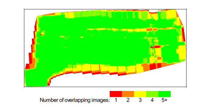
The quality report also provides a diagram showing how much overlapping imagery there is throughout a mission.  Figure 8, below, displays these areas. 

figure 8: amount of image overlap for cannon SX260

Referring back to figure 8, the areas with the lowest amount of overlap are at the bottom and to the right of the image.  The low number of overlapping imagery was likely known before the mission, and was allowed because it was not of high importance to the grand scheme of the mission.  Had the mission done one more pass over these given areas, the amount of overlap would be higher than what we currently can see. 

GEMS

figure 9: GEMS specs and quality check 

Here in figure 7, above, one can view the GEMS specifications and the quality check conducted after the initial processing process of the Pix4D project  creation.  Of the 146 images input for this this project, 142 were able to be calibrated and used to create the orthomosaic and DSM.   After examining the data in Pix4D, the area where there is no calibrated imagery is a wooded area of dispersed trees and other vegetation.  This is likely the case because trees are very dynamic in their shape, trajectory, and pattern, and would thus be very poorly represented. 

Relating those images that were not calibrated to wooded areas, let us observe the overlap diagram produced by the quality report for this project in figure 10 below.

Overall, there is a very high degree of overlap for almost the entire area.  However, with that being said, there are are areas outside of the edges of the mosaic that have poor overlap.  The areas being referred to are the right-central location and a the thin line that crosses the upper portion of the AOI.  relating this to the orthomosiac produced, both these portions that resemble areas of poor overlap are forested areas, and are not represented in the final orthomosaic, they are blank spaces blotted through out that area.  

Comparing the two projects, the GEMS mission has a much more dense level of overlap compared to that of the Cannon SX260 mission.  This is not a comment on the sensors capability, but is refering too the difference in mission planning that likely took place.  The area of interest for the GEMS mission is much more dynamic and changing, and thus would require more overlap to create an accurate orthomosaic and DSM.

For a video tour of these areas of poor data quality due to low overlap ratio, click here.

Ray Cloud: Measuring Areas and Distances in Pix4D

The ray cloud tool utilizes the multiple angles and distances of the various images  taken to provide accurate 3D areas and distances of user created polygons or lines.  The key for this tool to be accurate, is having the same area as overlapped from different angles and distances as possible.  Here are a few a measurement oppertations conducted using the data produced with the Cannon SX260. These measurement features were later exported to ArcMap, and are apart of the maps compiled later on in this lab assignment

Line Measurement
Line measurement is a helpful tool for both applying the software, and quality checking data. In this instance, the tool was used to measure a straight portion of a track which has a known length of 100 meters.  Going from line to line, the results were as such:

Terrain 3d length: 100.60 M
Projected 2d lengh: 100.55 M

The discrepancy between the distance recorded and the actual distance of the track (100 M) is likely due to the distorted pix-elation that occurs at close levels when zoomed at high levels onto the track.  Figure 7 shows what is meant by this with an example of the distortion.

figure 7: distortion of cannon SX260 point clouds in Pix4D

Area Measurement

Measuring the area of a given space is also a helpful tool made available through the rayCloud tool. After an area is created, a toolbar on the right shows the multiple angles the area created can be seen through the vantage point of the different images that have an overlapping viewing area of the same portion of the surface.  Using these images, the user can subsequently alter the vertices of the polygon the polygon they created.  Here are the specs of the area captured in the middle of the open field next to the track at South Middle School. 

Enclose 3d area: 705.50 square meters 

Projected 2D area: 656.72 square meters 

Here is the area which was recorded and produced theses values.

figure 8: area captured using rayCloud in Pix4D 

Volume Measurement  

The final thing that one can do using rayCloud is calculate interval volume measurements of areas or items that are apart of your surface.  The volume value can either be positive or negative, indicating weather the the mass of the measured feature a divet in the surface or something that occupies space above the surface.  Similar to what you can do with the vertices in area measurements, the user can also view the feature they created in all of the images that overlap that area of the surface, and can subsequently alter the vertices as they see fit.  The area measured for this example was a drainage ditch-like divet between an open field and the parking lot.  here is what this area looks like and its subsequent volumetric measurements.

Fill volume: -41.37 meters cubed (+/- 5.45)

Total volume: -40.94 meters cubed (+/- 5.85)

figure 9: volume area of a drainage ditch processed in Pix4D

Final Maps 

by exporting these maps to Arcmap, the files ore oriented and can me made into maps.  Figure 10 and 11 below show the maps made from the GEMS and Cannon SX260, in that order.

figure 10: GEMS mosaic

Figure 11: Cannon SX260 mosaic

Conclusion 

Pix4D is a powerful software with very useful open source capabilities.  Being able to upload imagery from a wide array of sensors and subsequently process the data within those images into a product that can be used for any number of applications across a wide range of various industry needs is what sets it apart from other software, like that of the GEMS, which we have already worked with. Software with GEMS, is only very useful when working with GEMS hardware. Pix4D, on the otherhand, may have a few more user inputs required to create meaningful results, but is a much better tool for someone who is more verse in remote sensing with imagery captured from a UAS.  The results produced were of high quality, and most importantly, through using the software i was able to gain a better understanding of the technological nuances of creating orthomosaics and DSMs. 

Lab 2: Using GEMs Processing Software - A Reveiw.

Introduction

As an introduction to the specifications of this software and hardware, Dr. Hupy provided students with manuals that in detail describe the hardware and software used in GEM products.  In essence, GEMs is a custom sensor intended for use in UAV applications .  Along with these manuals, students were given questions intended to provide enough guidance to the point we would then be able to process imagery using GEMs products and actually be able to understand what is actually being created and review the products of the operations conducted. 

GEMs Hardware

What does GEMs stand for?

GEMS stands for geo-locating and mosaicing system.

Look at figure 3 in the hardware manual and name what the GSD and pixel resolution are for the sensor. Why is that important for engaging in geospatial analysis. How does this compare to other sensors?

GSD: 5.1 cm at 400 feet - 2.5 cm at 200 feet

Pixel Resolution: 1.3 mega pixels

This information is important for geo-spatial analysis because how much ground is covered per pixel provides information of how large something must be on the ground in order for one to definitively identify what is they are seeing. Other sensors, like the Cannon SX260 HS, shoots images with 12.1 MP and has a GSD of  2.2 cm at 200 ft / 5 cm at 400 ft.

How does the GEMs store its data?

The hardware creates a Flight Data Folder per flight mission.  That folder is than extracted by the software as a FlightData.Bin File. Within that file is the trajectory of the flight, metadata, and geo-acurate tiffs are stored.  Being in the same file location makes it easy for the technology to run quick operations like mosaicing and NDVI initialization.  All the files that are created from operations conducted in the software are also stored within the same FlightData.bin file.

What should the user be concerned with when mounting the GEMs on the UAS?

When installing the GEMS payload, it is imperative to do a number of things or there is a risk for damaging the hardware, or producing poor quality data.  The payload should be mounted on the bottom of the plane, flat, at least 4 inches away from magnetic material (i.e. engines or batteries), and must be properly secured to limit vibrations.  Also, the anetena should be wired so that they are away from any significant sources of EMI.  One way to limit this interference on multirotors is  wiring the antenna to be above the propeller rotors.

Examine Figures 17-19 in the hardware manual and relate that to mission planning. Why is this of concern in planning out missions?

Some of the concerns with mission planning are anticipating how GSD, image blurring, and amount of overlap are attributed from different mission planner variables.  varying levels of speed and height require different degree of image overlap to create accurate mosaics. Going at a faster speed also increases the amount of movement distortion at lower heights.  To create a full array of robust imagery, its important to understand your subject area and how much overlap will be needed to create a good product. 70% overlap is desired for quick stitching, but working with percents closer to 50% is possible if working with images containing distinct features that in each image that would assist in aligning the images.  Doing missions over agricultural land, where the surface is relatively featureless, it would be more appropriate to employ a higher degree of overlap.

Write down the parameters for flight planning software (page 25 of hardware manual). Compare those with other sensors such as the  Cannon SX260, Cannon S110, Nex 7, DJI phantom sensor, and Go Pro?

One thing that is apparent when comparing the specs of the other sensors like the Cannon SX260 or a GoPro is the lower level of picture quality.  Many of these sensors twice the amount of pixels density on a larger sensor, meaning that there is both more pixels and each pixel is self is smaller.  The SX260 for example had pixel size of 1.54 x 154 micro meters to the GEMs 3.75 x 3.75 micro meters.

Table 1: Specs of GEMS and Cannon SX260 sensors.

GEMs Software

Read the 1.1 Overview section. Then do a bit of online research and answer what the difference between orthomosaic and mosaic for imagery (orthorectified imagery vs. georeferenced imagery). Is Sentek making a false claim? Why or why not?

An orthomosiac is a more advanced version of a georeferenced image. For an image to be referenced, each pixel must have an attributed x and y dimension, its only in one dimension. Orthomosiaced images are georeferenced in 3 dimensions, they have an associated z value for each pixel as well. According to the manuals presented by Sentek Systems, there is no sensor that is apart of the GEMs system that is able to collect a point cloud containing elevation data. The GEMs sensor only collects in visible spectrum and near IR.  To create a Orthorectified image, one has to use software to combine georefrenced imagery with a digital surface model that was recorded with 3rd, separate sensor. Doing this allows for the data product to accurately extract precise sloping and distance information, which is impossible with a georefrenced image.

What forms of data are generated by the software?

The data generated by this software are images showing RGB, Near IR, NIR of the areas captured during a flight mission.  Attributed to each pixel of these images, are 2 dimensional GPS coordinates.

How is data structured and labeled following a GEMs flight? What is the label structure, and what do the different numbers represent?

The files are saved under a labeling system comprised of GPS time syntax.  The names generally look like this: (Week=(####) TOW=(######).  Using a converter from the this sight, a file that looks like Week = 1862 TOW = 135349 would represents the standard dating/time system as 2015/09/04 6:35 and 32 seconds, Central Time.  GPS time is a continuous, non-repainting counting system  that counts weeks  starting from January 5, 1980.  the first four digits represent the number of weeks since that date and the digits after TOW (time of the week) represent the number of seconds that have passed since midnight of the previous Sunday.

What is the file extension of the file the user is looking to run in the folder?

The file saved under the GPS dating system is a .bin file.

Methods

What is the basis of this naming scheme? Why do you suppose it is done this way? Is this a good method? Provide a critique.

For the sake of organization, the first thing that will be done is changing the file names to the standard dating system. Using a converter from the, a file that looks like Week = 1862 TOW = 135349 would represents the standard dating/time system as 2015/09/04 6:35 and 32 seconds, Central Time.  GPS time is a continuous, non-repainting counting system  that counts weeks  starting from January 5, 1980.  Although this file syntax system has advantages for scripting, it is unlikely anybody seeing this timing method will be able to make sense of it in quick simple way like they would with a standard timing system. Employing this scheme is tedious outside of scripting operations because Sentek Systems does not provide any sort of conversion apparatus, and the one that is referenced above proved to be hard to find, it would be nice if they offered a conversion calculator of some sort.

Explain how the vegetation relates to the FC1 colors and to the FC2 colors. Which makes more sense to you? Now look at the Mono and compare that to the vegetation.

 Figure 2: (Left to right) NDVI FC1 and NDVI FC2. 

Given that that NDVI images pertain to vegetation health, the FC1 opption to me would make the most sense given its green to red scale. Green representing healthy vegetation, and red representing unhealthy vegetation or areas lacking vegetation, that color scheme translates well to the common sense that most people attribute to the what each color represents, if they know that the imagery is classifying varying levels of vegetation.

Figure 3: Display scale for Mono-chromatic images

Similar to the scale of the NDVI FC2 referenced in figure 3, the mono scale shows healthy vegetation in lighter shades and areas with unhealthy/no vegetation as darker.

Do these produce orthorectified images? Why or why not?

The two type of mosaics are fast mosaics and fine mosaics.  The only difference between the two is that the fine mosaic performs additional computer vision image processing operations, and takes a little bit longer to process.  Again, these are not orthorectified because they have not attributed elevation data.

Describe the quality of the mosaic. Where are there problems. Compare the speed with the quality and think of how this could be used.

The quality of the mosaics are good enough, but than could easily be improved if ran with fine mosaicing.  It did not take long at all to run a quick Mosaic which poses an advantage for field for conducting field work.  Provided you have a strong enough computer system, this running quick mosaics is possible in the field, allowing for the data to be check on site for quality and accuracy.  Later on, fine mosaics could be ran to create a better product, which in itself does not take much longer than quick mosaics, especially when using a device where GPU processing can be enabled.

The only area where there is a little bit for distortion in the image are near the overlapping areas near the edge of the newly mosaiced image, where you see edge forming between the images composing the mosiac.  There seems to be less of this issue in areas with more contrasting features, near the center of the mosaic.

Navigate to the Export to Pix4D section. What does it mean to export to Pix4D? Run this operation and look at the file. What are the numbers in the file used for?

Exporting the bin files to Pix4D allows the user to actually conduct orthorectification processes, if elevation data is available. Also, exporting a bin for Pix4D creates an excel table for NDVI FC1, NDVI FC2, Mono, and RGB.  Each excel table contains the central coordinate taken when each image was taken in lat and long, as well as columns containing the  Alt, Omega, Phi, Kappa values of each image. within these tables, it would be nice if each column was labeled so the viewer could know the what type of values they are looking at without having to refer to the software manual.

What is a geotif, and how can it be used?

A geotiff is an image that contains geographical accurate pixels, that is the picture itself, and each of the pixels, has an associated GCS x and y coordinate. This feature allows viewers to locate very accurately, in 2 dimensions, where a given feature is.  The geotiff. file structure is completely open source, which it allows it to be opened up, imported, and operated on by a number of different software programs like GEMs, Pix4D, and Arcmap.

Go into the Tiles folder and examine the imagery. How are the geotifs different than the jpegs?

In comparison, viewing the image as a tiff vs. jpeg doesn't produce any noticeable difference.  With that being said, the geotiff files are much larger than the jpeg files due to the geospataial data that is stored with the actual imagery.

Results 

Now open Microsoft Image Composite Editor software and generate a mosaic for each set of images. What is the quality of the product compared to GEMs. Does this produce a Geotiff? Where might Microsoft Image Composite Editor be useful in examining UAS data?


 Using the Mono from the JEMs imagery folder, ice creates a panorama file of all the images you select (in this case, all mono images).  The panorama was very smooth and showed no visible level of distortion that i could see.  To the right of the viewer there are a number of projection options that allow you to alter the shape and orientation of the panorama in several ways.  However, since this does not provide accurate coordinates for each picture/pixel, it is not a geotiff.  It does however, allow for the use of combining JPEG images into one, high quality panorama.  This could be useful for pure viewing purposes when just aiming to to create a high quality images by just combing jpeg taken during a flight.

Microsoft's ICE software allows users to make panoramas out of JPEG files taken during flight.  after running NDVI operations, this can be done for the RGB, NDVI FC1, NDVI FC2, and Mono files that were created using the GEMs software.  Although the output is not geolocated, it still created a very nice and seamless mosaic, as you can see in figure 4.  One issue when creating these panoramas and exporting them as JPEGs is that the file size becomes too large to import into blogger, so the image you see below is a screenshot taken with snip-tool. because it is a screen shot, the quality of the image is lower than the original file created in ICE.

figure 4: Panorama created from Mono - RGB jpegs from UAV flight.

To utilize the GEMs for its intended agricultural purposes, let us look at the the NDVI FC2 georefferenced mosaic and contrast it with the results obtained from the ICE software.  Figure 5 below shows a map of the of the same area, but was created using fast mosaic operations in GEMs.

figure 5: Maps created from GEMs hardware and software

Viweing these maps, it is apparent that there is a high amount of distortion and poor data quality at throughout these mosaics.  This perhaps is due to the fact that fine mosaicing operations were not initialized.  IF you look at the False Color 1 map, the distortion is very apparent when you focus on the northern portion of the image and see how broken up the lines of the soccer fields are.

GEMs Hardware and Software Conclusive Review 

Although the sensors apart of the GEMs payload do not have the highest resolution, for the purposes of precision agriculture, its enough.  The sensors are not designed to take high quality photographs that are able to produce aesthetic maps or diagrams, they are manly intended to detect varying degrees of vegetation species and health. The software and hardware is very simple, light, and easy for first time users to use without having a very deep understanding of remote sensing because the hardware and software are very intimately integrated.  All it takes is a load and a few clicks and data product desired is produced with little to know user input.

The GEMS sensor hardware is limited though because it does not have a very wide field of view, and thus requires that more paths be ran by a UAV in order to capture the full area of interest.  This can be a problem when the device being used has a battery life of 30 minutes, it limits the amount of data one can actually collect.    What is also missing from the software is the ability of it integrate point cloud data that would provide Z values which would allow for the creation of true Orthomosaics.

Overall, the software and hardware provided for GEMs is good enough for the application it is intended for, precision agriculture, but it lacks diverse applications that has become common place in modern technology.  To vastly improve upon this platform, it would be wise to consider investing in technology that upgrades resolution of the image, and perhaps incorporating a sensor that can collect ground level z values, so that true orthomosaics can be made.

As a teaching tool, this software provided great insight on the basic operations that can be done one remote sensing data collected from a UAV platform, highlight how nice it is to work with technology that has highly integrated software and hardware.

Sources:

Sentek hardware and software manuals

GPS time converter: https://dominoc925-pages.appspot.com/webapp/calc_gpstime/

Lab 1: Constructing Maps with UAS Data

Introduction

One of the most sought after skills in the world of UAS are those who can process imagery data that has been collected and compile the data in maps that are easy to read and understand by people outside of the industry.  As a practicing geographer, simply posting pictures of areas should be avoided at all cost, and any time we do post a picture an image it should be tide together with a map that contains a spatial reference, north arrow, and a legend. The following activity is an introduction of how to process data collected from a UAS device, interpret patterns, and describe those patterns in a concise way.  This activity will be conducted in a template format, where a question provided to us from Dr. Hupy will be posted in bold letters and the subsequent answers below them in normal font.

Methods

In this section, students will be copying and pasting a folder into your own student folder that contains a series of examples of UAS data. Each bullet will be a section on working with the data and creating maps from that data. You will then have questions that you will paste into your report with an answer.

Flash Flight Logs

Flash Flight Logs are KMZ files that represents that different executed maneuvers of a UAV mission.  The file is broken up in terms of the different behaviours of the device i.e. loitering vs auto-pilot flight.

What components are missing that make this into a map?

In this view, we see the flight path of two different paths composed by a few different layers that correspond to the specific activity associated with the device during a certain portion of its flight.  To make this a map, there would need to be a scale representation of some sort, a north arrow for directional reference,  and a legend to tell viewers what it is they are seeing. Without these items, there is no spatial context to refer to, which in geographic terms, is something you never want to allow.

What are the advantages and disadvantages of viewing this data in Google Earth?

Viewing this data in Google earth has advantages and disadvantages. In terms of advantages, it is very quick and simple, which is good if one only wants to get a quick glimpse at a flight path, especially if they are already familiar with the nature of the flight and what it was conducted for.  In terms of disadvantages, however, in google earth you can only view the physical path/height of the path, and no other attributed information that would otherwise be available if you opened the program.  Such elements like a scale bar, north arrow, or a legend, the essential elements for creating a map, are not available, which means you cant present this data in any sort of professional or educational setting with any level of credibility.

how do you save a kmz file as a kml file?  

Right click on the the 'flight path auto' layer and chose to save to my places as.... You then go to the location you wish to save the file and change the file type to kml instead of kmz, which are your only two options.

Go into ArcMap, bring in imagery base data, and import the kml into ArcMap. How do you do this?

There is a tool called KML to Layer.  It was used and the output location was my lab folder in the Q drive. The subsequent map can be seen in figure 1 below:

Figure 1

Telemetry Logs

Telemetry Logs is a file created during the flight of a UAV when using Mission Planner software. The telemetry log file contains detailed information about speed, pitch, yaw, and other components that were apart of a mission.

Use Mission Planner to convert a Tlog into a KMZ (How do you do this?)

When mission planner is opened up, the home interface has a set of tabs on the left side of the screen, one of those tabs is a tool labled 'Tlog > Kml of Graph'. This tool allows you to do a number of things, but in this instance, it was used to created a KML out of a telemetry log. The subsequent file created is a KMZ file that includes multi-path, multi-point, and multi-patch elements. Using the same 'KML to layer' tool used in the Flash Log conversion.  The resulting map shows the layer created from that telemetry log based KMZ file.

Figure 2

 GEMs Geotiffs

A geotiff is a raster file where each cell is geolocated.  Along with the pixel, the file contains all the information needed to place cells in their accurate locations based on different mapping projections and datums

Add each of the GEM Geotiffs into ArcMap. Build Pyramids and Calculate Statistics for each file. What does calculating statistics allow you to do?

Calculating the statistics for any raster based file allows for you to subsequently reclassify the raster layer to show the prevalence of different cell values.  In this case, the cell values represent varying levels of the electromagnetic spectrum.  The data was collected through the use of varying sensors mounted on a UAV device.  Figure 3, below, shows the 5  Geotiffs in conjunction with one another, after having their statistics calculated in ArcMap.

Figure 3

Pix4d Data Products 

Pix4d data products use unique software to conducted advanced photogrammetric operations to be conducted on raster data collected by UAVs. Using the software, one can create orthorectified images (orothomosiacs) as well as digital surface models (DSMs).

What is the difference between the DSM and the Orthomosaic?

A digital surface model is raster data set that models the earth surface, including the objects that are on top of the terrain.  Attributed to each cell is the height of surface for the given area the file covers. In contrast, an orthomosiac is composed of multiple raster files mosaiced into one image that covers a given area.  These combined rasters are orthorectified to remove any distortion by means of projecting the data in a coordinate plane, and apply z values to the the image, removing distortion caused by scale variation. Once this process is complete, the entire image looks like the photo was taken from a sensor directly above.  This opperation is done by combining multiple images that slightly overlap each other.  Meanwhile, A DSM need only one snap shot of the surface to gather the information necessary for that given area.

Go into the Properties for each DSM and record the descriptive statistics for each. What are those statistics? Why use them?

These calculated statistics tell us the min, max, mean, and first standard deviation for the totality of the cells that make up the DSM raster file.  This information could be use in comparative circumstances, where one wanted to compare the same area at different times.  Linking those changes to where they occur on the image would than give you a good indication how that areas landscape is changing.  Is the entire area losing top soil from erosion (lower mean)? Or is there a pile of sand that keeps on growing (higher max)? Knowing these values and having two points of comparison over a given time period allows you to process the information and reach conclusions about what changes are occurring in a specific landscape

Hillshade the DSM images. How did you do this? Delineate regions of the DSM, thinking of each region in terms of topography, relating that to the vegetation.

To apply a hillshade to a DSM all one must do is go to properties - - symbology, and check the box next to 'use hill shade effect'.

Open ArcScene and bring in the DSM and Orthomosaic for flight 2 of sivertson mine. Then set the base ht to the dsm. Display the ortho in 3D, along with the DSM. Explain what this information needs to become a map. How might one do that? That is, list out the criteria needed for this to become cartographcally correct.

In order to turn this newly created 3d surface model into  map, one would need to apply the essential map elements that provide the spatial context that need to be apart of its presentation as a credible map.  Such elements include north arrow, scale indicator, legend, and a title. Because this is a 3d model, however, applying a scale becomes difficult because you have varying surface heights which means there is no constant scale, it is varying depending on surface height.  One thing that you could do is apply a fishnet over the surface, where each full grid-square represents the same amount of area.  Squares closest to the viewepoint will be larger than those further away from the viewpoint will be smaller, eventhough they cover the same amount of area. figure 4 below exemplifies this type of scaleing.

figure 4

Results

T-Logs: In reference to figure 1, above, the pattern illustrated by the flight log 'auto-pilot' path has the characteristics of a multirotor.  For instance, if you look at the flight path you notice that the turns are very sharp and square.  To describe this, the device takes long north/south trips, turns on a sharp right angle to the east, goes for roughly 30 meters, and then returns to its north/south path.  In total, the flight ran 4 north/south runs, and the end of the forth, the device stopped and turned back and went directly back to the starting point of the flight.  If this flight path was that of a fixed wing that, the turns would be much more rounded and would likely take 60 until the device was completely going the opposite direction from whence it just came.  The 30 meter gap between the north/south runs conducted by the multirotor indicate that this flight was done at relatively higher altitude.  If the flight was conducted lower to the ground, there wouldn't need to be such large gaps between the north/south runs because the device would have to move a shorter distance to ovoid producing an unnecessary overlap in the images being taken.

Geo-Tiffs: How does the RGB image differ from the base map imagery. What is the difference in zoom levels? How does this relate to GSD?

The RGB geotiff from the GEMproducts file provides a much more rich and contrasting tones and colors in comparison to the ArcMap basemap imagery. If you zoom into the border areas where the geotiff ends and all there is is the background basemap imagery, one can see that the geotiff retains a much higher level of detail at closer zoom levels. In terms of a ground sampling distance, because the pixel size is smaller you could use a smaller object to create a scale reference for your image.

What discrepancies do you see in the mosaic? Do the images match seamlessly? Are the colors 'true' Where do you see the most distortion.

Within the the geotiff it's hard to see the detail in portions of the image where the surface has a brighter surface or lighter color associated with it. This image, shows the surface of the AOI in true color, in that the image shows the RGB colors of the ground surface. There are also a few places where the overlapping areas seem to contrast slightly in brightness, and don't flow seamlessly into the next frame.

Compare the RGB image to the NDVI mosaics. Explain the color schemes for each NDVI mosaic by relating this to the RGB image? Discuss the patterns on the image. Explain what an NDVI is and how this relates.

NDVI = (near infrared - visual light)/(near infrared + visual light)

A NDVI is also known as a normalized difference vegetation index.  The index is often created on a scale of -1 to 1 where values closest to -1 are water and values approaching 1 are healthy, lush vegetation. The color scheme used to symbolize an NDVI is subjective to the user, as they can classify it depending one what values they want to highlight.  In the file NDVI-FC1, we see color scheme contrasting from bright red to dark blue.  In contrast to the RGB image, the areas with red are are the areas of the RGB image which are heavily shadowed and the areas that are darkest blue are the roads.  reclassifying the mono NDVI shows that areas with the highest NDVI value are the areas with shadow, and the lowest values are the road and random areas throughout the vegetation.  This pattern remains consistent in each mosaic.

The shadows  show high NDVI values because there is little or no visible light being emitted from that area, but near IR is still present.  Transversely, in areas like the road wither you have very low values, the concrete is very light and thus is giving off a high amount of both RGB light as well as near IR.  The healthy vegetation within the garden can be seen by values giving off high near IR values, which is an associated quality of healthy plants, they absorb most visible light and reflect a large amount of near IR wavelengths.

Orthomosiac/DSM: What is the difference between an orthomosaic and a georeferenced mosaic?

An orthomosiac are a series of images that have been combined into one image and also orthorecitified to remove overhead distortion.  Subsequently, each pixel is precisely geolocated in both the X,Y and Z plane. This is done by mosaicing images with at overlapping points and combining that mosaic with a point cloud in the from of a digital surface model file, providing elevation values as well as XY coordinates. A georefrenced mosaic is an orthorefrenced mosiac but it has no DSM as apart of it, and thus has no Z values.  As a result if you were to use a georeferenced mosaic to calculate the distance between two points, you would get an inaccurate measurement because the distance calculation would only take 1 dimension into consideration.

What types of patterns do you notice on the orthomosaic and DSM. Describe the regions you created by combining differences in topography and vegetation.

To area of interest, Litch Field Mine, has a number of different of regions based of of both land cover and topography.  Below, in figure 5, one can explore a map showing the distinctive regions of this site

Figure 5

Refering to the map in figure 5, much of the areas with higher topographic features are composed of man made piles of unknown materials.  The areas of higher topography are marked by 3 distinct regions and are labeled by their relative cardinal direction.  Of all the pile regions, the only area that seems to contain piles of a different material than the rest, is the east central region, where we see a pile of black material while the rest of the piles are composed of manily sandy colored material. Along the entire Northwest edge of the image frame, we see that there is a body of water, and opposite of that edge of the frame, to the south east, we see that there is a forested area.  Right next to the water body, in the center of the frame, we see what appears to be a drainage area, where any liquid that that remains above the surface would eventually flow toward, and ultimately end up in the water body we see at the edge of the frame. In that little drainage area, we see that there is a low level of vegetation growing.

Conclusion

The data presented in this lab report reviles alot of the unique aspects of collecting data with UAV mounted sensors. Traditional remote sensing practices relie on satelite imagery, which means in order to get highly detailed imagery of smaller areas, it is likely you have to repeatedly spend alarge amount of resources to acquire such data. With UAVs, the data collection of smaller areas becomes very specialized and hands on.  You can get a look at the ground surface on you own terms, and do a number operation on the information captured by the sensors that allow you to exemplify any number of characteristics you wish to highlight about that area.  The limitations associated with this UAV really depend on the device one is using.  Within the industry, different uav devices are specilized for certain things, and attempting to use a UAV for something that is not intended to be used for is not a wise thing to do.  Therefore, when working with UAV based data is important to know the specific hardware used both for the data collection and flight operations. As we did in this lab, using this data in correlation with some sort of credible refrenced imagery or basemap provide assurance to users that the data that they are working with is accurate and  usable.  Going forward, it will be important to keep these aspects of UAV data in mind while collecting, and processing the data available